A paper titled Neural Ordinary Differential Equations proposed some really interesting ideas which I felt were worth pursuing. In this post, I’m going to summarize the paper and also explain some of my experiments related to adversarial attacks on these networks, and how adversarially robust neural ODEs seem to map different classes of inputs to different equilibria of the ODE. I reached this conclusion by playing around with the time over which the ODE is solved, and then looking at how they respond to adversarial attacks. Before I go into these experiments, here’s a summary of the central ideas proposed in the paper.

Paper Summary

The primary idea in the paper is that neural networks can be thought of as dynamical systems with each layer corresponding to propagation by a single time step. We can then extend this idea to continuous time – or a notion of continuous layers to form networks with an “infinite” number of hidden layers.

From ResNets to ODEs

The central concept clicked in my mind while reading the insightful explanation in this thread by senior author David Duvenaud. The key insight is to start from residual networks, and extend the notion of discrete layers to a “continuum” of layers over time, which manifests as an ordinary differential equation, or ODE.

Residual networks differ from standard deep networks in that they attempt to learn the change in hidden activations instead of learning a direct transformation. Functionally, we can represent this as follows, with $x$ as an input and $f_i$ as neural network layers:

$z_1 = f_0(x) + x$

$z_2 = f_1(z_1) + z_1$

$z_3 = f_2(z_2) + z_2$

$z_4 = f_3(z_3) + z_3$

Where the $z_i$ are hidden activations. If we look carefully, this looks awfully similar to how the Euler Method would solve an ordinary differential equation. The “time” variable in the ODE is equivalent to layer number or “depth” in this context. Rewriting the above equations in a slightly different way might make this more apparent:

$z(t=0) = x$

$z(1) - z(0) = f(z(0), t=0)$

$z(2) - z(1) = f(z(1), t=1)$

$z(3) - z(2) = f(z(2), t=2)$

$z(4) - z(3) = f(z(3), t=3)$

It’s clear now that the change in hidden activations (or state) $z$ over layer depth (or time) is given by the dynamics defined by the function $f$. It’s a function (which is a neural network) of both the activations and the depth (analogous to general ODE dynamics depending on both state and time). We can now go to the continuous domain and write an ODE:

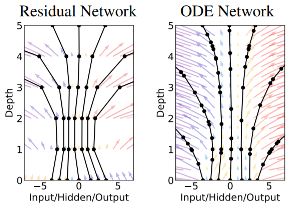
\[\frac{dz}{dt} = f(z(t), t; \theta) \label{n_ode}\]

Where $\theta$ denotes the parameters of the neural network. When this ODE is solved using Euler’s method, we retrieve our ResNet equations. Now, if we just start from this ODE, we don’t have to solve it by the Euler method. We can use general (and better) ODE solvers like Runge-Kutta methods. This is the central idea of Neural ODEs. The diagram below might help to make the analogy between ResNets and ODE-nets clearer:

Advanced ODE solvers differ from the simple Euler method in multiple aspects:

• They are higher order methods, meaning they perform multiple function evaluations for each step of solving the ODE (which leads to more accurate solutions).
• More importantly, they have adaptive step-sizes, which means that they don’t find the solution at fixed time intervals like the simple Euler method, but at varying time intervals based on how complex the dynamics are. This is where the analogy with ResNets starts to depart, because ResNets simply add the output of the “dynamics” at each “time step” (or layer), meaning that the difference between each layer is a fixed time interval. However, ODE-nets can evaluate the hidden activations or state at varying time intervals adapting to the complexity of the dynamics. The diagram in the paper brings out this difference well:

What about backprop?

Backprop can, in theory, be performed through all the operations of the ODE solver and this can be used to train the model. This however, requires writing differentiable versions of the ODE solvers we use. A neat trick to avoid this is presented in the paper – the adjoint method. In essence, it extends the standard chain rule used in backprop to a continuous version, which leads to another ODE.

Suppose our ODE-net solves the neural ODE from time $t_0$ to $t_1$. Our loss function $L$ takes in the final state $z(t_1)$ as its input. Assume that we know its gradient $\frac{dL}{dz(t_1)}$ as well. Let us try to find the gradient of the loss with respect to the state at any time. This is defined as the adjoint state $a(t)$:

\[a(t) = \frac{dL}{dz(t)}\]

Note that $a(t)$ is taken as a row vector to avoid writing transposes everywhere. If we know this gradient at all times, we can simply use the chain rule to find the gradient with respect to the neural network parameters $\theta$, by summing up the contributions of each time step going backward. In the continuous domain, this amounts to an integral:

\[\frac{dL}{d \theta} = \int_{t_1}^{t_0} a(t) \frac{\partial f(z(t), t; \theta)}{\partial \theta} dt\]

Note that this is a hand-wavy explanation, and I have shoved some intricacies under the rug.

But how do we find the adjoint state? Well, this requires some slightly involved math, so buckle up. If you want to skip the derivation, go to the last paragraph of this section for the final result. The derivation I’m about to present is based on the proof in Appendix B of the paper.

First, we need to better understand the transformation that the ODE-net is performing:

\[z(t_1) = z(t_0) + \int_{t_0}^{t_1} f(z(t), t; \theta) dt \label{theta_grad}\]

We can break this up into a composition of infinitesimal transformations $T_\epsilon$, each of which advance the state $z$ by some tiny amount of time $\epsilon$:

\[z(t+\epsilon) = z(t) + \int_{t}^{t+\epsilon} f(z(\tau), \tau; \theta) d\tau = T_\epsilon(z(t), t) \label{T_eps}\]

Now we can apply the chain rule on these infinitesimal transforms to get:

\[\frac{dL}{dz(t)} = \frac{dL}{dz(t+\epsilon)}\frac{dz(t+\epsilon)}{dz(t)}\]

Equivalently by substituting from $\ref{T_eps}$,

\[a(t) = a(t+\epsilon) \frac{\partial T_\epsilon(z(t), t)}{\partial z(t)} \label{chain_rule}\]

Now, the derivative on the right hand side is the jacobian of the infinitesimal transform $T_\epsilon$. From $\ref{T_eps}$, we can first use the fact that $\epsilon$ is small and Taylor expand around $z(t)$ to get:

\[T_\epsilon(z(t), t) = z(t) + \int_{t}^{t+\epsilon} f(z(\tau), \tau; \theta) d\tau \approx z(t) + \epsilon f(z(t), t; \theta)\]

Now, we can easily find the jacobian as:

\[\frac{\partial T_\epsilon(z(t), t)}{\partial z(t)} \approx I + \epsilon \frac{\partial f(z(t), t; \theta)}{\partial z(t)}\]

Substituting into $\ref{chain_rule}$, we get:

\[a(t) \approx a(t+\epsilon) \left(I + \epsilon \frac{\partial f(z(t), t; \theta)}{\partial z(t)}\right)\]

Rearranging,

\[\frac{a(t+\epsilon) - a(t)}{\epsilon} \approx -a(t+\epsilon) \frac{\partial f(z(t), t; \theta)}{\partial z(t)}\]

Finally, we can let $\epsilon$ go to $0$ and notice that the left hand side is a time derivative:

\[\frac{d a(t)}{dt} = -a(t)\frac{\partial f(z(t), t; \theta)}{\partial z(t)}\]

This is now just another ODE, which we can solve using any ODE solver to obtain the adjoint state. Well, what about $z(t)$? We can just recompute it for the required time points by solving the original ODE $\ref{n_ode}$ backward. Along with the integral in $\ref{theta_grad}$, we need to solve a total of three ODEs to find the gradients with respect to $\theta$. This can be done with one call to an ODE-solver by just augmenting the three states together, and defining one combined augmented dynamics. We can now go ahead and train our ODE-net without worrying about the specifics of our ODE-solver!

Benefits of ODE-nets

ODE networks have some really useful properties:

• They are much more memory efficient compared to conventional ResNets. An ODE-net achieves the same performance as a ResNet on MNIST classification with roughly 3 times fewer parameters.
• An aspect I haven’t talked about is tolerance or error in ODE solvers. ODE solvers take a tolerance level as an argument while solving, which controls how accurate the solution is at the cost of more function evaluations. This can be used as a tradeoff between performance and speed. For example, ODE-nets can be trained with very low tolerance values which can be later relaxed at test time for faster inference.
• The variable time step aspect can be used for continuous time-series models, unlike RNNs which have inputs at fixed intervals of time.
• Possibly the most impactful benefit is in continuous normalizing flows. A high level description is that the continuous nature of the ODE-net as opposed to a discrete network greatly simplifies and speeds up certain computations in training. I won’t go into more details now, as this topic deserves a whole post on its own.

Connections between Adversarial Robustness and Equilibria

While the above applications are very interesting, I experimented with a much simpler aspect of the ODE network, the integration time. We saw earlier that the ODE is solved from some time $t_0$ to some time $t_1$ with the input as the initial state, and the output taken as the final state. In the implementations of the networks in the paper, the authors only used a start time of $t_0=0$ and an end time of $t_1=1$ for their classification networks, as far as I’m aware. For brevity, I’m going to refer to the end time as just $t$ and drop the subscript.

In my experiments, I tried out different schemes for choosing the end time. One of them was to just increase it to something like $t=10$ and $t=100$. Note that this doesn’t increase the parameters of the network as those are present only in the dynamics given by the function $f$. Another interesting method was to choose a random end time between $t=10$ and $t=100$ each time the ODE-net is called. I thought that this stochasticity might enforce some form of robustness by forcing the ODE to settle to an equilibrium. This network indeed showed a slight increase in accuracy on adversarial inputs, but only for a smaller sized ODE-network with roughly $17k$ parameters. I also performed these tests using a larger network with around $655k$ parameters. Both the networks had the same architecture, but the larger one had more channels in the ODE state. I’ve summarized the results into a table below. The accuracies shown are on standard/adversarial test datasets, with different end times while testing. I used a basic Fast Gradient Sign Method (FGSM) attack on the cross-entropy loss for creating the adversarial test examples.

Network	Training end time	t=1	t=10	t=100	t=500
ODE-net small	10	49.45 / 0	98.64 / 9.34	26.35 / 12.83	9.94 / 8.09
ODE-net small	10-100	61.54 / 0	98.46 / 0.52	98.31 / 23.64	94.35 / 11.67
ODE-net small	100	37.58 / 0	66.43 / 0	98.52 / 13.25	72.16 / 14.16
ODE-net large	10	97.06 / 0.18	98.93 / 30.76	91.43 / 28.20	9.35 / 8.57
ODE-net large	10-100	72.84 / 0.15	99.08 / 70.67	99.11 / 85.98	94.66 / 62.29
ODE-net large	100	78.88 / 0.59	98.85 / 83.13	99.01 / 92.62	96.68 / 78.60

Some notable observations:

• The larger network consistently had better adversarial accuracies than the smaller one. This is in accordance with section 4 of this paper by Madry et. al. which shows that networks with more capacities are generally more robust to adversarial attacks.
• However, training the network for larger end times also improved robustness. This indicates that capacity alone is not the deciding factor for adversarial robustness. It seems like the end time, which somewhat corresponds to network ‘depth’ might also play a role, however the definition of the depth of an ODE network is not clear.
• Using the random end time method improved the results only for the smaller network, but just using $t=100$ worked out better for the larger network. The effect of capacity might have won over the randomness while training, but the larger end time still played a role even for the larger network.
• The smaller network when trained using the random end time method retained its performance for much larger times like $t=500$, while training it with just $t=100$ didn’t perform as well in normal tests. This effect is not present for the larger ODE-net, where both training schemes had persistent performance for a large time range beyond what they were trained with. Nevertheless, this phenomenon indicates that the state of these networks probably settles to some sort of equilibrium, or changes very slowly as time progresses even beyond what they were trained with.

Apart from messing around with end times while training, I also adversarially trained an ODE network and tested it with different end times. Adversarial training is basically a form of data augmentation in which the added data points are just adversarial examples. This means that adversarial examples are generated on the fly while training and the model is then trained to correctly classify them as well. This leads to adversarially robust models. It also had some other interesting results for ODE-nets:

• Adversarial training led to much larger function evaluations for the same end time. Normal training for $t=1$ usually had $20$-$30$ function evaluations, but adversarial training for the same end time had function evaluation counts in the $100$s. This probably indicates that the dynamics are more complex, but I couldn’t make a rigorous conclusion from this result.
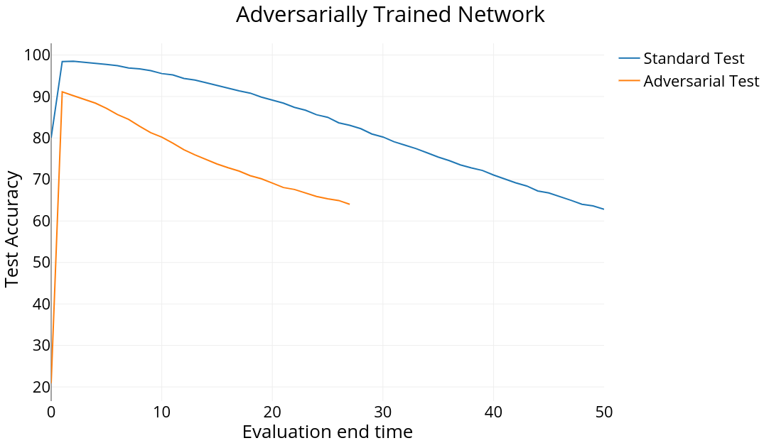
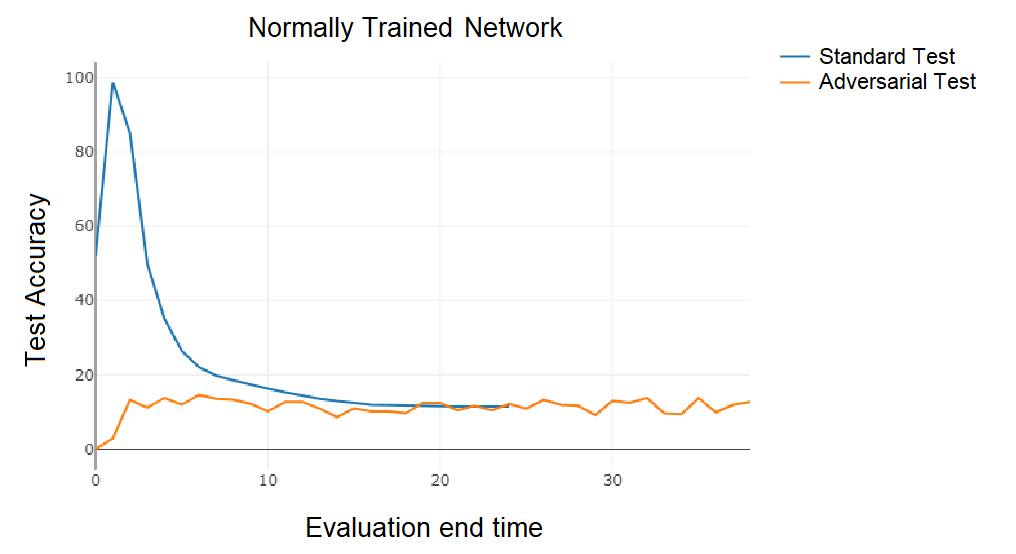
• Adversarially trained ODE networks exhibited much better performance for further end times than ones which weren’t trained adversarially. This probably means that these ODEs settle to some sort of equilibrium which is unique to the class of the input (because the subsequent fully-connected layer is still able to distinguish between the final states) and adversarial inputs are also pulled towards these equilibria. The graphs below show the performances of the two networks for a range of end times.

We can visualize the state of the ODE-net evolving through time to get a better idea of what’s going on. Note that, to display the state as an image, we have to normalize the values of the state to the range $[0,1]$, so it’s not a completely faithful representation of the state, though it will still provide some insight into the dynamics.

It seems like the adversarially trained ODE state settles down faster than the normally trained one. At least I couldn’t perceive significant changes in it when compared to the normal state. On closer inspection, I discovered that the state does in fact change by growing in scale, so the normalized image appears constant. This actually means that the derivative of the ODE state, the neural network $f$, is a constant. So it is technically not in ‘equilibrium’, but in a steady-state of sorts because the derivative state is itself in equilibrium.

I performed the same visualization for two different input digits, over a much larger time-scale so that the steady state becomes more apparent.

It’s clear that adversarial training has probably made the ODE create different steady states for different input classes. This, however, is just an intuitive explanation of what might be going on under the hood, and a more rigorous analysis is definitely needed. Looking at neural networks from a dynamical system point of view could provide really insightful explanations of their behavior and I definitely believe that this is a direction worth pursuing with more rigor and careful analysis. I’d love to hear your thoughts on this subject, so go ahead and tweet me @rajat_vd.

You can find the code I used for this project in this github repo. I also used a neat package which the authors of the neural ODE paper released for differentiable ODE solvers using the adjoint method called torchdiffeq.

References

1. Neural Ordinary Differential Equations. Ricky T. Q. Chen, Yulia Rubanova, Jesse Bettencourt, David Duvenaud. NeurIPS 2018.
2. Towards Deep Learning Models Resistant to Adversarial Attacks. Aleksander Madry, Aleksandar Makelov, Ludwig Schmidt, Dimitris Tsipras, Adrian Vladu. CoRR 2017.
3. For an explanation of adversarial attacks like FGSM - Explaining and Harnessing Adversarial Examples. Ian J. Goodfellow, Jonathon Shlens, Christian Szegedy. ICLR 2015.

---

I’d like to thank the Computer Vision and Intelligence Group of IIT Madras for generously providing me with the compute resources for this project.