Animating Doodles with Autoencoders and Synthetic Data

In this post, I’m going to go over a recent project of mine in which I trained some autoencoders on synthetic data created by randomly painting lines and curves on an image. I also created a bunch of animations by interpolating in latent space between some of my crudely drawn doodles. I tried out different interpolation methods to make various types of animations.

The Synthetic Dataset

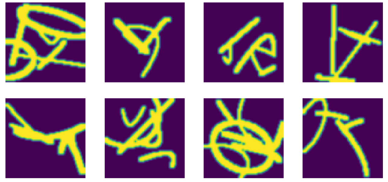
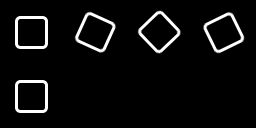
The dataset I trained the autoencoders on was a synthetic dataset, which means that the data is programmatically created. This type of dataset is different from normal datasets in that it isn’t collected or annotated in anyway. In essence, the dataset is created in the computer itself. The particular synthetic dataset I used consisted of grayscale images (64x64) with random lines, curves and ellipses painted on it. A random number of each of the shapes are painted with random attributes:

Lines - random endpoints.
Bezier curves - random endpoints and anchor point.
Ellipses - random centres, rotation and eccentricity.

Each of the shapes is also painted with a random stroke width. Here are some samples from the dataset:

sample from dataset — Some sample images from the synthetic dataset. Note the variation in number of strokes, stroke width and types of strokes. The vast number of possibilities makes the size of this dataset huge.

The Autoencoder

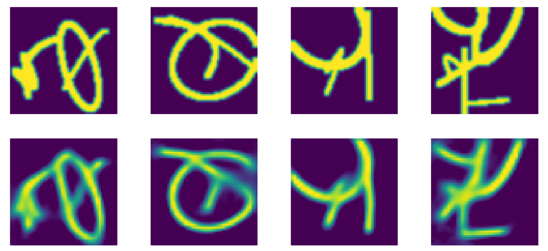
The first model I trained used a convolutional encoder and decoder with residual connections. The networks were fairly deep with around 20 conv layers for both the encoder and decoder. I experimented with different sizes for the latent space encoding, and ended up using 64. The model performed pretty well, here are some inputs and outputs:

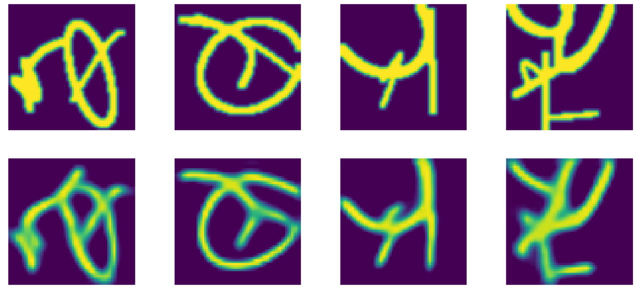
convconv sample — Input images (top) and the corresponding reconstructions (bottom) made using an autoencoder with conv layers and residual connections. We can see that the reconstructions fail to capture finer details, and are also more blurred out compared to the inputs. However, they manage to recognize many of the strokes correctly.

I also tried out the CoordConv layer described in this paper. It basically just adds a meshgrid of $x$ and $y$ coordinates as 2 more channels in the input image. This adds a spatial bias to the conv layer. I couldn’t find much quantitative difference in terms of training speed or final performance, and nor could I notice much qualitative changes in the outputs:

coordconv sample — Input images (top) and the corresponding reconstructions (bottom) made using an autoencoder with CoordConv layers. Similar problems as the previous case exist, as it fails to reconstruct finer details in crowded parts of the input image.

Interpolation and Animation

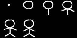
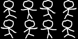
Now for the fun bit. Using the autoencoder I just described above, I interpolated between some doodles I drew up in paint. The process is quite simple:

Given a sequence of grayscale images, pass each of them through the encoder of the trained autoencoder.
Linearly interpolate between the encodings of each image sequentially.
Apply the decoder on each of the interpolated points and string together the resulting images to form an animation between the input images.

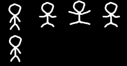
This produces interesting animations which pay attention to the characteristics of strokes and curves in the images. Here is one such animation which shows a tree-like structure growing from a point.

tree images — The input sequence of images of a growing tree-like structure, and the resulting animation obtained by interpolating between them in latent space. Note that the reconstructions aren't perfect, with some of the finer details missing.

tree interp 0 std — The input sequence of images of a growing tree-like structure, and the resulting animation obtained by interpolating between them in latent space. Note that the reconstructions aren't perfect, with some of the finer details missing.

Apart from a basic linear interpolation, I also tried to use a circular interpolation. This is done by first linearly interpolating between the euclidean norms of the two encodings to get a set of interpolating norms. Then, each of the vectors obtained by normal linear interpolation between the two encodings are scaled to have norms equal to these corresponding norms. It turned out that this didn’t make much of a difference. Another interpolation method which produced better qualitative results involved adding some randomness to the process.

Brownian Bridge Interpolation

I added a brownian bridge to the path obtained by linearly interpolating between two encodings. A brownian bridge is a random walk which starts and ends at the same value (in this case, $0$). A simple way to generate a brownian bridge is as follows:

Generate a gaussian random walk. Let’s call this sequence of vectors $X_t$, where $0 \leq t \leq 1$ is the time index of the points in the walk.
To make the brownian bridge $Y_t$, we just do the following:

\[Y_t = X_t - t X_t\]

Now that we got a random walk beginning and ending with 0, we can add this to each of the interpolating paths between the input images. Here’s the same tree animation as above, with added brownian bridges using different standard deviations for the random walks:

tree std 0.3 — Animations obtained by adding brownian bridges of standard deviations 0.3 (left) and 1.3 (right) to the interpolating paths in latent space.

tree std 1.3 — Animations obtained by adding brownian bridges of standard deviations 0.3 (left) and 1.3 (right) to the interpolating paths in latent space.

The added noise in the interpolating paths manifests as shaky animations as opposed to noise in the actual image. The encoding in the latent space is sort of a compressed representation of the input image, with information about the curves and strokes in the image. So, adding noise to this encoding will result in perturbations in properties of the lines and curves, making them look shaky. Qualitatively, these animations seem a bit more realistic than the plain linear interpolations.

Here are some more animations I made and their corresponding input image sequences. Compare the ones with and without the added brownian bridge.

jj images — Input images for a jumping jack animation. The animation clearly shows upward motion as the stick figure jumps.

jj std 0 — Input images for a jumping jack animation. The animation clearly shows upward motion as the stick figure jumps.

man images — Creating a stick figure from a point. The brownian bridge noise really makes the animation more interesting as the one without noise (left) seems too artificial.

man std 0 — Creating a stick figure from a point. The brownian bridge noise really makes the animation more interesting as the one without noise (left) seems too artificial.

sq images — If the input images are sufficiently close together, objects can also be made to rotate.

sq std 0 — If the input images are sufficiently close together, objects can also be made to rotate.

brain images — The autoencoder can successfully reconstruct English alphabet as well. This can be used to make animated words like this one.

brain std 0 — The autoencoder can successfully reconstruct English alphabet as well. This can be used to make animated words like this one.

neuron images — The interpolations between some of the letters are quite interesting.

neuron std 0 — The interpolations between some of the letters are quite interesting.

walk images — My crude attempt at trying to make a stick figure walk. Seems more like a dance move though.

walk std 0 — My crude attempt at trying to make a stick figure walk. Seems more like a dance move though.

The above animations look pretty realistic, but the reconstructions are far from perfect. Training an autoencoder with a different architecture could possibly make them sharper and more accurate. It would also be interesting to use other types of models like disentangled VAEs to try to extract meaningful features out of the learned encodings like stroke width, curve position, etc.

This fun little project goes to show that you can use deep learning to make cool stuff even if you don’t have a dataset to play with - just make your own!

Cubic Spline Interpolation

Addendum on Aug 4

Some of you suggested to try out higher order interpolation techniques as they might result in smoother animations. Indeed this is a great idea, so I went ahead and made some gifs using cubic spline interpolation. Here are some of the gifs with the linearly interpolated ones as well for comparison:

dance std 1.2 — The gif created using cubic spline interpolation (right) seems smoother compared to the one on the left.

dance cube 0.5 — The gif created using cubic spline interpolation (right) seems smoother compared to the one on the left.

walker std 1.0 — Although the differences in the above examples are much more subtle and hard to make out.

walker cube 0.8 — Although the differences in the above examples are much more subtle and hard to make out.

neuron std 0.8 — It's almost the same in the case of letters as well.

You can find my code for this post here. It’s written using pytorch, with the aid of some utils I made. Special thanks to my brother Anjan for the discussions we had about the ideas in this post.

Written on August 2, 2018